STAT 302, Lecture Slides 8

class: center, title-slide

# STAT 302, Lecture Slides 8
## Resampling
### Peter Gao

---

# Outline

1. Permutation Tests
2. Bootstrap

.middler[**Goal:** Understand various computational approaches for statistical inference.]

---
# Motivation

Suppose we want to examine the oft-cited claim that right-handed people live longer than left-handed people. We randomly sample 10 left-handed and 10 right-handed death certificates and compare the sample average lifespans. Suppose we find that the right-handed sample mean is 3 years longer than the left-handed sample mean.

What is our null hypothesis here?

`$H_0:\mu_{L}=\mu_{R}$`

The **sample mean difference** of 3 years is an example of a sample statistic. We want to know: Is this difference meaningful, or is it just noise? What should we do?

---
# A parametric approach

A common approach here is the **two-sample t-test** for difference of means. Can we use this method here? What assumptions does this test require?

--
Usually:

1. Observations must be **independent** of each other.
2. Each population should be (approximately) normally distributed.

Are these assumptions satisfied?
---
# A parametric approach

The t-test relies on our being able to construct a test statistic with a t-distribution. If our assumptions are met, then our test statistic should have the right distribution.

![](08_resample-bayes_files/figure-html/unnamed-chunk-1-1.png)
---
# Another approach?

However, this is not the only hypothesis test we could use here. Consider that our data looks something like this:

If our null hypothesis is true, there should be no relationship between age at death and handedness **in our sample**. We can sample from the null distribution by randomly assigning handedness to our data points and calculating the resulting sample statistic.

---
# An example with actual data

```r
library(ggplot2)
# experiment comparing growing conditions' effect of growth
data(PlantGrowth)

ggplot(PlantGrowth, aes(x = weight, fill = group)) +
  geom_histogram() + facet_wrap(~group) + theme_bw()
```

![](08_resample-bayes_files/figure-html/unnamed-chunk-3-1.png)

Is there a difference between Treatment 2 and Control?

---
# The t-test

```r
t.test(x = PlantGrowth$weight[PlantGrowth$group == "ctrl"],
       y = PlantGrowth$weight[PlantGrowth$group == "trt2"])
```

```
## 
## 	Welch Two Sample t-test
## 
## data:  PlantGrowth$weight[PlantGrowth$group == "ctrl"] and PlantGrowth$weight[PlantGrowth$group == "trt2"]
## t = -2.134, df = 16.786, p-value = 0.0479
## alternative hypothesis: true difference in means is not equal to 0
## 95 percent confidence interval:
##  -0.98287213 -0.00512787
## sample estimates:
## mean of x mean of y 
##     5.032     5.526
```

---
# A permutation test

```r
# remove treatment 1
PlantGrowth <- PlantGrowth %>%
  filter(group != "trt1")
obs_diff <- mean(PlantGrowth$weight[PlantGrowth$group == "trt2"]) -
    mean(PlantGrowth$weight[PlantGrowth$group == "ctrl"])
obs_diff
```

```
## [1] 0.494
```

Is this difference meaningful?

---
# A permutation test

```r
# store permuted differences
permuted_diff <- numeric()
for (i in 1:10000) {
  # for each iteration, scramble group variable
  permuted_data <- PlantGrowth %>%
    mutate(group = sample(group))
  # compute difference
  diff = mean(permuted_data$weight[permuted_data$group == "trt2"]) -
    mean(permuted_data$weight[permuted_data$group == "ctrl"])
  # store difference
  permuted_diff[i] <- diff
}
```

---
# A permutation test

```r
hist(permuted_diff)
```

![](08_resample-bayes_files/figure-html/perm.1c-1.png)

How do we compute a p-value?
--

```r
# calculate p-value
mean(abs(permuted_diff) > abs(obs_diff))
```

```
## [1] 0.0472
```
---

# A permutation test for correlation

Suppose we have two variables, `x` and `y`, and we want to test whether they are correlated. What should we do?

We could use some sort of parametric test, or ...

---

```r
set.seed(1111111)
sim_data <- data.frame(x = rnorm(11),
                       y = c(rnorm(11)))
plot(sim_data)
```

![](08_resample-bayes_files/figure-html/perm.2a-1.png)

```r
cor(sim_data$x, sim_data$y)
```

```
## [1] -0.108006
```
---

```r
# store correlations
permuted_cor <- numeric()
for (i in 1:10000) {
  permuted_data <- 
    data.frame(x = sim_data$x,
               y = sample(sim_data$y))
  permuted_cor[i] <- cor(permuted_data$x,
                         permuted_data$y)
}
```

---

```r
hist(permuted_cor)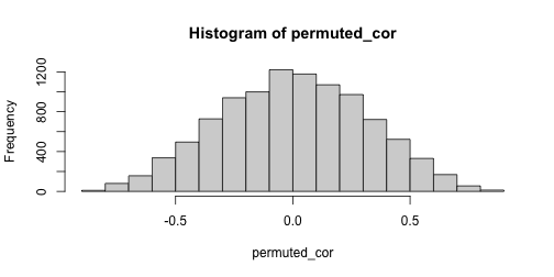
```

![](08_resample-bayes_files/figure-html/perm.2c-1.png)

```r
# calculate p-value
mean(abs(permuted_cor) > abs(cor(sim_data$x, sim_data$y)))
```

```
## [1] 0.7433
```
---
# A wonkier example

```r
set.seed(1111111)
sim_data <- data.frame(x = rnorm(11),
                       y = c(rnorm(10), 20))
plot(sim_data)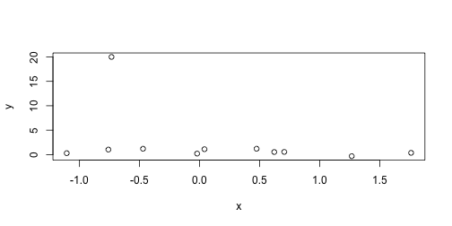
```

![](08_resample-bayes_files/figure-html/perm.3a-1.png)

```r
cor(sim_data$x, sim_data$y)
```

```
## [1] -0.3603595
```
---
# A wonkier example

---
# A wonkier example

```r
hist(permuted_cor)
```

![](08_resample-bayes_files/figure-html/perm.3d-1.png)

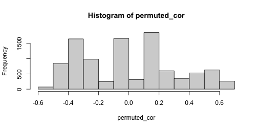```r
mean(abs(permuted_cor) > abs(cor(sim_data$x, sim_data$y)))
```

```
## [1] 0.2988
```

---
# Bootstrap

Suppose we sample 25 houses in Seattle and get their sale prices. How can we construct an interval estimate for the mean house price of all houses in Seattle?

```r
library(moderndive)
data("house_prices")

# population mean price
pop_mean <- mean(house_prices$price)

set.seed(1234)
sample_prices <- sample(house_prices$price, size = 25)
(sample_mean <- mean(sample_prices))
```

```
## [1] 550689.3
```

---
# Bootstrap

Assuming independence and approximate normality, we can construct a t-interval:

```r
t_res <- t.test(sample_prices)
t_conf_int <- t_res$conf.int
t_conf_int
```

```
## [1] 438403.5 662975.1
## attr(,"conf.level")
## [1] 0.95
```
--

```r
hist(house_prices$price)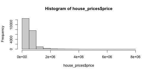
```

![](08_resample-bayes_files/figure-html/unnamed-chunk-7-1.png)

---

# Bootstrap

We can use resampling to construct what is called a bootstrap confidence interval. Essentially:

1. Resample with replacement from our existing sample many times.
2. For each resample, compute the resample mean. 
3. Take the 2.5 and 97.5 quantiles of the resample means.

```r
bs_sample_prices <- as.data.frame(sample_prices) %>% 
  rep_sample_n(size = 25, replace = TRUE, reps = 10000)
bs_sample_means <- bs_sample_prices %>%
  group_by(replicate) %>%
  summarize(bs_mean = mean(sample_prices))
bs_conf_int <- quantile(bs_sample_means$bs_mean, probs = c(.025, .975))
```

---
# Bootstrap interval

Below we plot a histogram of our bootstrap means.

```r
hist(bs_sample_means$bs_mean)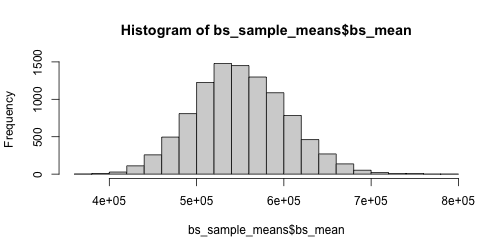
```

![](08_resample-bayes_files/figure-html/unnamed-chunk-8-1.png)

```r
bs_conf_int
```

```
##     2.5%    97.5% 
## 450801.7 658507.4
```

---

# Comparing bootstrap and t

```r
set.seed(1234)
t_conf_ints <- matrix(ncol = 2, nrow = 1000)
bs_conf_ints <- matrix(ncol = 2, nrow = 1000)
for (i in 1:1000) {
  # initial sample
  sample_prices <- sample(house_prices$price, size = 15)
  # t-interval
  t_res <- t.test(sample_prices)
  t_conf_ints[i, ] <- t_res$conf.int
  # bootstrap interval
  bs_sample_prices <- as.data.frame(sample_prices) %>% 
    rep_sample_n(size = 15, replace = TRUE, reps = 10000)
  bs_sample_means <- bs_sample_prices %>%
    group_by(replicate) %>%
    summarize(bs_mean = mean(sample_prices))
  bs_conf_ints[i, ] <- quantile(bs_sample_means$bs_mean, probs = c(.025, .975))
}
```

---

# Comparing bootstrap and t

```r
mean(t_conf_ints[, 1] < pop_mean &
       t_conf_ints[, 2] > pop_mean)
```

```
## [1] 0.91
```

```r
mean(bs_conf_ints[, 1] < pop_mean &
       bs_conf_ints[, 2] > pop_mean)
```

```
## [1] 0.897
```

---
# Recap: Why resample?

--
1. Existing parametric methods rely on assumptions
2. Resampling methods can leverage computational power to help us avoid making inappropriate assumptions.